2D Panel Cutting
2D Panel Cutting is CutOptim’s primary mode. It solves the classic rectangle bin-packing problem: given a set of large rectangular sheets and a set of smaller rectangular pieces, find the arrangement that uses the fewest sheets with the least waste.
This mode is used for sheet materials including plywood, MDF, particleboard, melamine, glass, aluminium composite panel, steel sheet, foam board, and any other material that comes in flat rectangular stock.
How 2D Optimization Works
CutOptim models your cutting job as a bin-packing problem:
- Bins are your stock sheets — large rectangles you are cutting from
- Items are your demand pieces — smaller rectangles you need to produce
Rather than filling in a single greedy pass, the optimizer runs several packing strategies over your whole job — different shelf and column layouts, sort orders and rotations — and keeps the best-scoring result (fewest sheets, least waste). Every strategy uses a guillotine cutting model:
- Guillotine cutting — Every cut goes edge to edge across the sheet. This mirrors how a panel saw, table saw, or beam saw works, so the resulting cut sequence is practical for manual and semi-automatic cutting. It is the 2D Panel mode’s cutting model; for true-shape (free-form) nesting of irregular parts — for CNC routers, laser, plasma or waterjet — use the separate Nesting mode.
CutOptim also respects kerf width — the material lost as sawdust in every cut. A 3 mm kerf on a 100-piece job can add up to losing an entire sheet. Always enter your kerf accurately. See Settings & Kerf.
Adding Stock Sheets
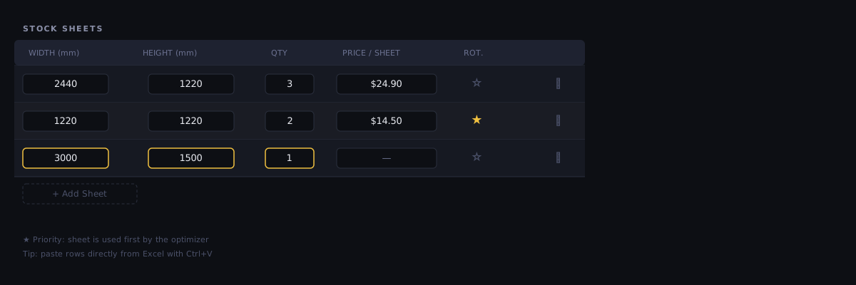
Stock sheets represent the raw material you have available to cut from. Each stock row defines one sheet size.
Sheet supply — the toggle above the table — decides how the quantities are read. In Unlimited (the default) the optimizer buys as many of each size as the plan needs, so a feasible job never fails for want of a board; the per-row quantity plays no part and its column is hidden. Switch to Limited only when you have a fixed number of boards on hand: each row’s quantity then becomes a hard cap, the optimizer combines your sizes to make everything fit, and the result names any pieces it could not cut. If a plan you know is possible comes back short, check that you are not in Limited mode with too few boards entered.
Several sheet sizes in Unlimited. When two or more sizes are entered, the optimizer also tries mixes of them — for example one large sheet fewer and one to three of a smaller size in its place — and keeps a mix only when every part still fits on less material. So the plan can use more sheets than before, but never more material.
Search harder for less material. When every part fits and two or more sheet sizes are entered, the plan offers Search harder for less material (usually under 15 s, at most 30 s) below How this plan was optimized. A stronger solver on our server looks for a mix of the sizes that uses less material — saw-cuttable layouts, and in CNC mode free layouts too. The plan changes only if every part still fits on less material; it is free and no run is charged. It is not offered with the Min. cost goal, in Material mode or with Grain matching sets.
| Feature | Type | Description |
|---|---|---|
| Width | number | Sheet width in the active unit (mm or cm). This is the horizontal dimension on the canvas. |
| Length | number | Sheet length in the active unit. This is the vertical dimension on the canvas. |
| Quantity | integer | How many sheets of this size you have. Shown and used only when Sheet supply is set to Limited, where it is a hard cap; in Unlimited (the default) the field is hidden and the optimizer uses as many sheets as needed. |
| Price | number | Cost per sheet. Used to calculate total material cost in the results summary and quotation export. Leave blank if pricing is not needed. |
| Name | text | Optional material name for this stock size, e.g. '18mm MDF' or '2400×1200 Structural Ply'. It labels the sheet on the plan and carries into the PDF and Excel exports, so the cut sheet says which board to fetch. Loading from the Material inventory or an offcut fills it in for you. |
Entering several sizes lets the optimizer combine them in one plan. If instead you are deciding which single size to buy, press ⚖ Which sheet? in the panel header: it runs your cut list on each size on its own and ranks them by material — see Which sheet? — comparing sheet sizes.
Best practices for stock sheets:
- Enter the actual usable dimensions of your sheet, not the nominal size. A sheet sold as 2440×1220 mm may actually be 2438×1218 mm after factory edge trimming — measure your sheets.
- If you have a mix of full sheets and partial offcuts from a previous job, add them as separate stock rows with their actual dimensions and a quantity of 1.
- Use the price field even for internal jobs. Seeing the cost breakdown helps identify whether a job is priced correctly.
Adding Parts
Parts are the rectangular pieces you need the optimization to produce from your stock. They go in the Parts (2D) table.
| Feature | Type | Description |
|---|---|---|
| Width | number | Required piece width in the active unit. |
| Length | number | Required piece length in the active unit. |
| Quantity | integer | Number of identical pieces required. |
| Label | text | Descriptive name for this piece, e.g. 'Door Panel LH' or 'Shelf 600'. Printed on the cut diagram and in the CSV export. |
| Grain (icon) | icon | Turn arrow (the default): the optimizer may turn the piece 90° to save material. Click once for lines across (grain along the Width), again for lines down (grain along the Length): the piece is placed with that side along the sheet's grain. The icon pictures the piece as entered; hover it for the exact side. The ⓘ in the header opens Grain Direction. Available on every plan. |
Tips for entering parts:
- Always enter a label for each piece. On a complex job with 50+ pieces, unlabelled rectangles on the cut diagram are impossible to identify.
- If you have many identical pieces, enter them once with the correct quantity rather than as separate rows.
- To add trim allowance (for pieces that need to be cut slightly oversize then trimmed to final size), set Oversize per side under Settings → More → Blade & trim and keep entering finished sizes. For example, a finished 400×800 mm piece with 5 mm oversize per side is packed and cut as 410×810.
CSV Import for Parts
If your cut list already exists in a spreadsheet, you can import it directly:
- Open the CSV ⌄ dropdown in the Parts section header (2D, 1D, or Wood) and choose Import CSV
- Choose your
.csvfile — columns are read by position:name,width,length,qty(an optional header row is detected and skipped) - The parts are added to the Parts table straight away
Not sure of the column order? Click the Template button next to the CSV import to download a ready-made CSV with the correct columns and an example row. See Importing data for the full reference.
Parts that must match: grain-matched sets
Under the Parts (2D) table sits the Grain matching strip (hide it with its ✕, and the Grain matching switch that then appears above the table, next to Edge Banding, brings it back). It appears once a part has a grain direction or is named like a door, drawer or front, or after a furniture template with fronts. It groups parts into a set — for example a drawer front over two doors — that is cut as one block: the parts side by side on the sheet, exactly one saw gap apart, with one grain direction, so the veneer figure runs on across them. A part in a set shows an A mark under its row number. Each part keeps its row in the table (sizes are still edited there); the set only says where the parts sit relative to each other. See Grain matching.
How CutOptim Cuts: Guillotine
CNC mode (since 14 October 2026). Everything in this section describes the default saw mode. If you cut on a CNC router, switch on CNC mode (free placement) in Settings: the parts are then placed freely, not on edge-to-edge cut lines — see CNC mode.
CutOptim’s 2D optimizer is guillotine-only — there is no cut-type toggle in Settings. Every cut is a straight line that runs from one edge of the (remaining) sheet to the opposite edge, mirroring the physical operation of a panel saw, table saw, or beam saw.
Why guillotine:
- The cut sequence can be handed to an operator as a straightforward cut list — or stepped through on screen with the Cutting Sequence player
- Works on a table saw, panel saw, track saw, or beam saw — no CNC required
- Cuts remain reproducible when material is flipped or moved between passes
Comparing against other tools: a free-nesting optimizer — one that drops pieces anywhere on the sheet — will usually report a higher yield than a guillotine optimizer on the same list. That gap is the price of cuts you can actually make on a panel saw, not a defect. Compare like with like before judging a number.
True nested (free-form) cutting — where pieces are placed anywhere on the sheet to squeeze out a few extra percent of yield on a CNC router — is not a cut-type toggle inside 2D Panel mode. For irregular polygons (and free-placed rectangles) use the separate Nesting mode; a rectangular free-nesting balanced engine is also available through the Engine API.
Cutting on a Panel Saw
A guillotine plan is only as good as the machine it is cut on, so six controls under Settings → More describe the saw rather than the material — Trim per side in Blade & trim, the other five in Cut plan & machine:
| Control | What it does | Modes | Plan |
|---|---|---|---|
| Trim per side | Dresses each edge of the board separately — left, right, top, bottom | 2D only (1D and Wood get the start / end trim pair instead) | Every plan, guests included |
| First cut direction | Forces the first cut on every sheet to run horizontally or vertically | 2D only | Every plan |
| Calibration cut | Skims a strip off one edge first, so you can measure it and correct the fence before cutting a part | Every mode — only the four-side picker is 2D, since a bar has one head | Every signed-in plan, Free included |
| Max. cutting stages | Caps how many times the material is turned — panel saws are specified as 2-, 3- or 4-stage | 2D only | Workshop |
| Minimise rotation | Prefers layouts that turn fewer parts, but only when that costs no extra sheet | 2D only | Workshop |
| Cut order | Lists the sawing plan per fence setting (panel saw, the default) or per pass (circular or track saw). Redraws the plan only: no new run | 2D only | Every plan |
Each one is documented in full on the Settings page. The finished order of cuts is then available as the Cutting Sequence, which steps through the plan one fence setting at a time — in every mode, not only here.
CutOptim does not produce machine-specific files — there is no .opt or G-code export, and DXF carries geometry only. What it produces is the plan, the numbers behind it and an order you can follow at the saw.
Running the Optimization
Once stock and parts are entered, click Run optimizer at the bottom of the left sidebar, or press Ctrl+Enter. The optimization typically completes in under 2 seconds for jobs with fewer than 500 pieces. Larger jobs take longer, and the page stays unresponsive until the calculation finishes.
What CutOptim checks before running: exactly one thing — that the active mode has at least one stock row and at least one part row. If either table is empty, a short message appears and nothing runs, so an empty run never costs you an optimization from your quota.
There is no other pre-flight validation, and nothing blocks the Run button. In particular, a piece too large for any of your stock will not stop the run: the optimizer simply cannot place it, and tells you afterwards — in limited-stock mode the result summary names every piece that did not fit. Quantity fields accept whole numbers from 1 upward and fall back to 1 if you clear them. (The plan allowance is separate from this check: when a Pro account has used its monthly runs with grain-matched sets and holds no credit, a run with sets stops and offers to run without them.)
Reading Your Results
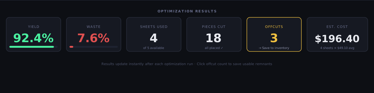
After a successful run, the canvas shows the layout and the results panel updates:
The sheet diagrams
Every sheet used is drawn one after another down the results panel, each under its own header showing the sheet number, the material name, the size, how many pieces it carries and how much of it is used. Placed pieces are coloured rectangles carrying their label and dimensions; a grain-matched set is outlined with a dashed frame and a SET A badge. The leftover material is listed under the diagrams rather than drawn on them, split into reusable offcuts and waste by your minimum offcut threshold.
The sawing plan on the results page
The results page adds two views of the order the cuts should be made in:
- The Cutting Sequence bar sits directly above the sheet diagrams it steps through — after the legend, before the first board — so the control and the boards it drives are in the same place on screen. It carries ◀ Previous, the step readout, ▶ Next, ⏮ Restart and ▶ Play.
- Further down, below the cut list, the whole plan is listed as a Cutting Sequence table: one row per fence setting, with the columns Order, Sheet, Cut direction (
horizontalorvertical, plus· Calibrationon the calibration step and· N passeswhere one setting makes cuts across N strips), Position and Result (what the step frees; for a multi-strip step per pass, such as3a → 27 · 3b → 28). Steps are numbered 1 to n on each sheet, not across the whole job. Clicking a row jumps the player to that step, and the active row is highlighted as you step through. If you saw with a circular or track saw, set Cut order to Per pass under Settings → More → Cut plan & machine and every cut becomes its own row.
See Cutting Sequence for the full guide, including how the plan looks on a bar in 1D and Wood.
Cuts, saw passes and cut length
Alongside yield, waste, sheets and pieces, a 2D result reports what the plan costs the saw. These stats are shown on every plan, guests included:
| Feature | Type | Description |
|---|---|---|
| Cuts | stat | Fence settings. Collinear cuts at the same coordinate made in the same machine pass count once, because that is one setup on the saw. This is the operator-facing number, and it is also the number of steps in the Cutting Sequence. |
| saw passes | sub-line | Shown under the Cuts figure when the two differ: every strip crossed separately. This is the number Cost per cut is charged on. |
| Cut length | stat | The total distance sawn — metres in mm mode, feet in inch mode. |
| Edge banding length | stat | Total running length of edge banding the parts list needs, shown only when at least one part has edges marked. Top and bottom edges run along the part's width, left and right along its height. It is exact geometry with no waste allowance — add your own margin for overlap and trimming — and it is broken down by banding type (a line per type plus an order total). Also printed in the PDF material requirement section and on the Materials tab of the Excel export, with a dedicated 'Edge banding by piece' page in the PDF and a dedicated Edge Banding tab in the Excel export — but never on the layout-diagram piece labels. |
The two counts are not alternatives and neither is wrong; they answer different questions. How many times do I set the fence? is the first. How many times does the blade go through material? is the second. On the standard 40-part demo job (2440×1220, kerf 3), the plan takes 30 cuts, 52 saw passes and 32.88 m of sawing across 2 sheets at 83.3% yield.
Cut length is the same figure under either counting convention, so it needs no qualifier. The search already prefers the shortest-cut plan among the layouts that use the same boards, which is why the demo comes out at 30 cuts by default. If your saw limits how many times the material can be turned, cap the Max. cutting stages (Workshop) — CutOptim keeps the plan within that limit where the job allows and warns you where it cannot, rather than handing back a plan the saw can’t execute (the demo job itself needs 3 stages).
Yield and Waste
| Metric | Formula | Target |
|---|---|---|
| Yield % | (Total demand area) / (Total used sheet area) × 100 | > 88% |
| Waste % | (Unusable scrap area) / (Total used sheet area) × 100 | < 10% |
| Offcut % | (Saved offcut area) / (Total used sheet area) × 100 | Variable |
Improving a Low-Yield Result
If yield is below 80%, try these approaches in order:
- Check kerf width — An incorrect (too large) kerf wastes space on every cut
- Allow rotation — Leave the Grain icon on the turn arrow for pieces where grain direction does not matter
- Batch more pieces — Add remaining pieces from future jobs to fill the sheets now
- Add smaller stock — If you have offcuts from previous jobs, move them into the stock table from the Offcut Inventory (↑ or All to stock): they are starred automatically and fill first
Stock Priority (★)
When Sheet supply is set to Limited, each row in the Stock table has a star (★) icon on the left — like the quantity, the ★ column appears only in Limited. Starring a stock row tells the optimizer to use that sheet first — before drawing from unstarred stock.
In Unlimited the ★ column is hidden and the star is not used: the optimizer buys as many sheets as the plan needs, so there is no stock to use up first. Your stars stay on their rows and count again when you switch back to Limited. Each row keeps its own star — the 2D, 1D and Wood stock tables are independent.
Off-cut rows. A piece you move into the Stock table from the Offcut Inventory (↑ or All to stock) becomes an off-cut row: it is starred automatically and is used first, never more than its quantity — in Limited and in Unlimited alike. In Unlimited it is filled before any new sheet is bought and is never repeated; a stock table made only of off-cut rows works like Limited, so no extra sheet is invented. The star’s tooltip on an off-cut row says so. An offcut you type in by hand is an ordinary row: to have it used first, switch to Limited and star it.
When to use it:
- You have a partial sheet left over from a previous job and want to use it up before opening new stock
- You have expensive or hard-to-source sheets that you want to prioritize
- You want to clear old stock before it warps or deteriorates
How to use:
- Set Sheet supply to Limited — the ★ column appears
- Click the ★ icon on any stock row — it turns yellow/gold
- Run the optimization — the starred sheet is used first
- Click again to remove the priority
Move your offcuts into the job from the Offcut Inventory (↑ or All to stock) instead of typing them in. They arrive starred, and CutOptim consumes them first, only opening new full sheets when the offcuts are exhausted — in either supply mode. With Use off-cuts automatically on, CutOptim reuses saved offcuts without any of these steps, in both modes.
Edge Banding
Edge banding is recorded per piece in the EB column of the Parts table: which sides of a finished panel are banded, and with which banding type. From that, CutOptim totals the linear metres of banding the job consumes, broken down by type.
Showing the EB column. The EB column is hidden until you switch edge banding on. In 2D → Panel mode, open the Settings panel, click More, and turn on the Edge Banding toggle — the EB column then appears in the Parts table and stays visible even after you collapse More again. Edge banding is included on every signed-in plan, Free included; a guest is prompted to create a free account. Edge banding applies only to 2D panels, so there is no EB column in the Nesting sub-tab, in 1D Linear, or in Wood mode.
Edge banding is a metadata/reference feature — it does not affect the optimization algorithm. It records which sides are banded and with which type, then reports the running metres so you can order the right amount of each banding.
Marking edge banding:
- Click the button in the EB column of any demand piece row.
- The edge banding dialog opens with an All around master control at the top, then the four sides: Top, Right, Bottom, Left.
- To band the whole piece at once — a door, say, that is banded on every edge — pick a type in All around and all four sides get it in one action (the master mirrors the sides, so it also shows the shared type when they already match). Otherwise set each side individually below.
- For each side, pick from the dropdown: None (not banded), No type (banded, no specific type), or one of your saved banding types.
- A visual preview shows the banded sides as a yellow stripe around the piece outline.
- Click OK — the EB column shows an abbreviation of the banded sides (
T/R/B/L).
EB column abbreviations:
| Display | Meaning |
|---|---|
— |
No edge banding |
T |
Top banded |
TR |
Top + Right banded |
TRBL |
All four sides banded |
BL |
Bottom + Left banded |
Banding types (library)
Click Manage types in the edge banding dialog to open your banding-type library. Each type carries a name (the reference you order by, e.g. ABS oak 22×1), a thickness, a price per metre and a colour — picked from a colour swatch, and used to draw that type’s edges in the per-piece banding diagram. Your types are stored to your account and sync across devices; assign them per edge from the dropdowns.
How the metres are reported
CutOptim measures the banded length exactly — top and bottom edges run the piece width, left and right run the piece height, multiplied by the quantity — with no waste margin (add your own overage at the bench). The per-type total appears in three places:
- The optimization summary — one figure per banding type.
- The PDF, in the material-requirement section, as a line per type plus an order total.
- The Excel export, on the Materials tab, as a row per type plus a total.
Beyond the totals, the banding is shown per piece in two places: the PDF has a dedicated Edge banding by piece page — each banded piece drawn with every edge in its banding-type colour and its length labelled, followed by a per-piece table of the material and length of each edge — and the Excel export has a dedicated Edge Banding tab with the same per-piece table plus a banding-layout picture.
Edge banding is still not drawn on the piece labels inside the layout diagram (the sheet plan) — those show dimensions only. It is printed on the part stickers: Share & Print → Print labels gives every banded piece an outline with the banded edges drawn thick and a line naming the sides and the banding type (since 2026-10-12). Beyond that, banding appears as the per-type totals above, plus the dedicated Edge banding by piece page in the PDF and the dedicated Edge Banding tab in the Excel export.
CSV
The Parts CSV has an EB column. Two forms are accepted:
TRBL— those sides banded, no specific type (any order, any case).T:ABS oak 22;L:ABS white 22— each named side takes that library type by name. Separate pairs with;(or quote the cell if you use commas). A name that matches no type still bands the edge (as No type), so nothing is lost.
For cabinet carcasses, a common configuration is BL (Bottom + Left) or TR (Top + Right) depending on whether the panel is a side, top, or shelf. Assigning the type once at the demand stage means the metre totals — and your order — are correct without re-checking at the bench.