How Cutting Optimization Actually Works — Methods Compared
Quick answer
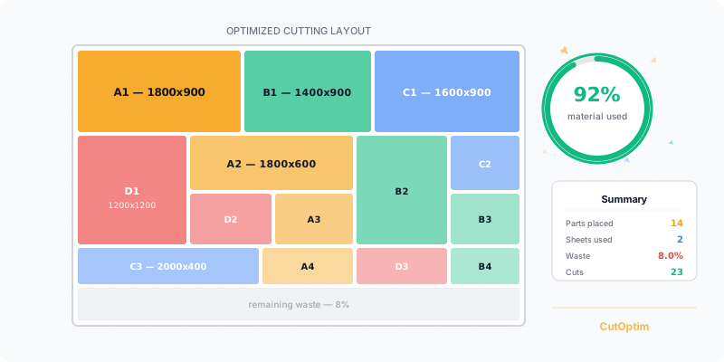
Cutting optimization arranges your parts on stock material to minimise waste, but the method matters more than the marketing. Guillotine optimizers only allow cuts that run edge to edge, because that is what a panel saw physically does. Free nesting places parts anywhere and can pack tighter, but its layouts often cannot be cut on a saw at all.
Run the same cut list through two tools and you often get two different numbers. Usually neither is smarter than the other: they solved different problems, and only one of the answers can be produced on your machine.
The Constraint Nobody Mentions First
A panel saw cuts edge to edge. The blade travels on a rail from one side of the material to the other, every time; there is no stopping halfway and restarting somewhere else without taking the workpiece off the machine.
That fact has a name in the literature: the guillotine constraint. Every cut must divide the current rectangle into exactly two rectangles, and you keep subdividing until each region holds one part. A layout containing parts that no edge-to-edge line can separate is not guillotine-cuttable — and on a panel saw it is not a plan, it is a picture.
Guillotine — every cut goes edge to edge
Six cuts, numbered in cutting order. Each one crosses the whole piece it is dividing, so the plan runs on a panel saw.
Free nesting — cuts that stop partway
The green cut is legal but has to stop halfway. Both red lines are edge-to-edge cuts, and each runs straight through a part.
This is why a “worse-looking” layout is often the only producible one. A guillotine optimizer throws away arrangements a free nester would happily keep, because keeping them would hand you a cut plan you cannot execute. Guillotine vs free cut nesting works through the geometry in detail.
“Another tool showed me a higher yield than you did.” Before concluding anything about software quality, ask what that tool assumed about your saw. If it nests parts freely — the normal mode for CNC routers, lasers and waterjets — it may place parts a panel saw cannot separate: its number is real for a CNC and unreachable on a sliding table saw. Kerf width, edge trim and per-part rotation also move the result, so compare those settings before comparing percentages.
The reverse is just as true: with a CNC router, a guillotine-only optimizer leaves material on the table. Neither approach is “better” in the abstract — they are answers to different machines.
The Method Ladder
Cutting optimization is a family of methods, not one algorithm. Knowing where a tool sits on this ladder tells you more than any yield figure it advertises.
1. Greedy heuristics
Sort the parts by a rule — largest area first, longest edge first — then place each one in the first position that fits. Shelf packing is the classic panel variant: build a band the height of the tallest part in it, fill it left to right, start the next band below. It is guillotine-valid by construction, which makes it a natural fit for saw work.
2. Multi-strategy best-of search
Instead of trusting one greedy rule, run many — several sort orders, several rotation policies, both possible first-cut directions, several packing families — score every resulting layout against an explicit objective, and keep the winner. The pathological input for one strategy is usually an easy input for another, so the worst case improves sharply even though no single strategy changed. This is the workhorse of practical cut-list software.
3. Metaheuristics
Simulated annealing, genetic algorithms, tabu search: rather than constructing one layout and stopping, these perturb a solution repeatedly, accepting some worsening moves to escape local optima. They keep improving after a constructive heuristic has run out of ideas — at the price of run time you cannot bound in advance, tuning that does not transfer between problem types, and, unless the random seed is fixed, answers that change between runs. That last one is awkward when the shop floor already has yesterday’s printout.
4. Exact methods
Formulate the problem as mathematics and solve it to proven optimality: mixed-integer linear programming, or constraint programming with a dedicated solver. The output is not “a good layout” but “this layout, and provably no better one exists” — or a bound telling you how much room is theoretically left. This is the only rung that can tell you when to stop looking.
The cost explodes with size: the cutting stock problem is NP-hard, so the search tree grows combinatorially with the number of parts and distinct sizes. Every real constraint — kerf, trim, grain, guillotine stages — also has to be written into the model, and each one added is more model to get right.
5. Pattern-based cutting stock (column generation)
The classic operations-research approach to industrial cutting, from Gilmore and Gomory (1961). Instead of deciding where each individual part goes, decide how many times to run each cutting pattern; because the number of possible patterns is astronomically large, you generate them on demand. It excels on high quantities of relatively few distinct sizes — rolls, bar stock, repeat panel orders — and buys little on a one-off job where nearly every part differs, because there is nothing to repeat.
6. Irregular (true-shape) nesting
A different problem class, not a harder rung of the same one. Parts are arbitrary polygons — curved furniture components, signage letters, gaskets, garment pieces — so the geometry itself becomes the hard part: deciding whether two shapes overlap at a given position and rotation, rather than comparing four numbers. The output is inherently non-guillotine and needs a machine that can follow an arbitrary toolpath.
| Method | What it buys | What it costs | Right when |
|---|---|---|---|
| Greedy heuristic | Milliseconds, fully predictable | No guarantee; fragile on odd part mixes | Simple jobs, or as one candidate among many |
| Multi-strategy best-of | Robustness across unknown part mixes | A constant multiple of one greedy run | Interactive cut-list software |
| Metaheuristics | Keeps improving past a single construction | Unbounded run time, tuning, non-repeatability | Large jobs where compute is cheaper than material |
| Exact methods | Proven optimality or a proven bound | Cost explodes with size; full model needed | Small part counts, expensive material, benchmarking |
| Pattern-based (column generation) | Strong results on repeat production | Assumes repetition; rounding of pattern counts | High quantities of few distinct sizes |
| Irregular nesting | Handles non-rectangular shapes | Heavy geometry; non-guillotine output | Shape cutting on CNC, laser, waterjet, plasma |
Notice what is missing from that table: a column of yield percentages. Any such number depends on your part mix, your stock sizes, your kerf and your rotation rules, so a figure copied from someone else’s job tells you nothing about yours. Judge a method by the guarantee it offers and the constraints it respects, then measure your own jobs.
What the Numbers Actually Mean
Optimizers report several numbers, and they answer different questions. Mixing them up is how people end up optimising for the wrong thing.
Material yield (%) is placed part area divided by the stock area consumed. It is the headline number and the one that ignores the most: it says nothing about how long the job takes to cut or whether the leftover material is any use. What material yield measures unpacks it further.
Sheet or bar count is usually the number that actually costs money — you buy whole sheets. A yield gain that does not remove a sheet from the shopping list may be worth very little; one that does can pay for itself immediately.
Cut lines and saw passes count the same plan two ways:
- A cut line is one fence setting — collinear cuts at the same coordinate in the same stage count once.
- A saw pass is one pass of the blade, counted separately for every strip it crosses.
CutOptim’s built-in demo job — 40 parts on 2440×1220 mm stock with a 3 mm kerf, fitting on 2 sheets at 83.28% yield — comes out as 30 cut lines and 52 saw passes: how often the operator repositions the fence, and how much sawing happens.
Sawn length is the total distance the blade travels through material. It is immune to counting conventions — merging collinear cuts on paper does not shorten the material — which makes it the fairest proxy for blade wear and cutting time.
A higher yield can cost you money
Two layouts can differ by a fraction of a percent of yield while differing substantially in:
- Setup time. More fence changes and more passes mean more minutes per sheet and more chances to mis-measure — on a short run, easily more than the value of the material saved.
- Offcut shape. Waste area is not waste quality. One layout leaves a clean rectangle you can rack, label and reuse; another leaves the identical area as a dozen thin slivers.
- Handling and stage count. A plan that needs more turns of the material is slower and riskier on large panels, regardless of how well it packs.
Pick the fewest sheets first, then the plan that is simplest to cut and leaves the most reusable offcut. Treat the last fraction of a percent of yield as a tie-breaker, not a goal.
Try It on Your Own Numbers
Generic yield figures are worthless, so here is the alternative. This is the guillotine multi-strategy packer described above, running in your browser on your own stock and parts.
For a full cut list with kerf, trim, offcuts and exports, open the optimizer. For a pre-set starting point, try the panel cutting optimizer or the board cutting calculator.
What CutOptim Does Today
The default, everywhere in the app, is a guillotine multi-strategy best-of search that runs in your browser — rung 2 of the ladder. No cut plan is uploaded anywhere to be computed.
The packer generates many candidates for your job — shelf packing and its transposed column form, across several sort orders and orientation policies, plus a straightforward greedy guillotine — then keeps the best by an explicit ranking: most parts placed, then fewest sheets, then most area used. First cut direction narrows that search when you need a specific orientation; cost mode re-ranks candidates by total stock price instead of sheet count.
Because every layout is guillotine-valid, the cut plan falls out of the finished layout: cut lines, saw passes, sawn length and stage count all come from the same reconstruction. That is what makes it executable on a panel saw rather than merely pretty. A job of around 2,000 parts solves on the order of a second on ordinary hardware — the measurement below puts one such job at ≈1715 ms.
Speed vs density: how hard to search
Most of that multi-strategy search is cheap, but one step — a per-board re-search that recovers the last few percent of yield on large, varied jobs — is expensive. A Speed vs density setting (an effort option on the Engine API) lets you skip that one step. Balanced, the default, runs the full search for the densest plan; Fast skips the expensive step, which is much quicker on large jobs for a few points less yield. Both stay fully guillotine-cuttable, and Fast is never denser than Balanced — it searches a subset of the same layouts, so it can only ever match or fall short, never beat it.
Measured on one demanding job — about 1,550 parts on a 2.07 × 5.6 m board — Balanced used 330 boards at 80.8% yield, and Fast used 350 boards at 76.2%, solving roughly 2.5× faster. On the small-to-medium jobs most shops run, the two are usually identical; the gap only opens on large jobs like this one.
These two — Fast and Balanced — are search depths on the guillotine optimizer above; both produce saw-cuttable plans. They are not the same thing as the separate balanced engine described next, which is a different (free-nesting) packer.
The opt-in free-nesting engine
Through the CutOptim Engine API, callers can opt into a second engine — balanced — which uses MaxRects free nesting instead of the guillotine search. It is for callers who want raw speed on very large jobs and can accept layouts a saw cannot cut. Measured on 2026-07-31, on a 2,000-part job:
| Default (guillotine, multi-strategy) | balanced (MaxRects free nesting) | |
|---|---|---|
| Speed on 2,000 parts | ≈1715 ms | ≈62 ms — about 25× faster |
| Yield on that job | 93.2% | 90.3% |
| Saw-cuttable layout | Always — every cut runs edge to edge | Often not guillotine-cuttable |
| Cut plan returned | Yes | Not when the layout is not guillotine |
Two things there are worth reading twice. The faster engine produced the lower yield on this job — free nesting is not automatically tighter; here the multi-strategy search simply searched harder. And balanced layouts frequently cannot be cut edge to edge, so the API reports them as not guillotine-valid and returns no cut plan at all. That is the trade you opt into deliberately, which is why the default never changes silently: the app’s optimizer is unchanged, and balanced runs only when an API caller explicitly asks for it. Both engines are documented in the Engine API reference.
An exact-optimisation mode is in development
New optimisation methods land in the Engine API before they land anywhere else — it is the surface where a caller can name an engine and accept its trade-offs. The next one is an exact-optimisation mode: instead of searching heuristically and returning the best layout it found, it proves optimality — this layout, with no better one possible, or a bound saying how much room is left. Rung 4 of the ladder above, offered as an engine.
It is in development and not available yet; heuristic and balanced are what the API serves today. It is an Engine API capability — the in-app optimizer stays on the guillotine multi-strategy search described above — and it is aimed at callers who will deliberately trade solve time for a provable answer: modest part counts on expensive material, or a benchmark to judge a heuristic against.
If you cut on a panel saw, you want the default and nothing else. The free-nesting engine is for API callers building their own tooling around machines that follow an arbitrary toolpath, or anyone who needs a rough packing answer on a very large job in milliseconds.
Choosing: A Short Decision Aid
Start with your machine. It removes most of the choice for you.
- Panel saw, beam saw or sliding table saw — guillotine, no exceptions. Optimise for fewest sheets, then fewest cut lines.
- CNC router, laser, waterjet or plasma — free nesting is usable, and worth it if your parts pack poorly under the guillotine rule. A guillotine plan still runs perfectly well here; it just does not use the machine’s full freedom.
- Both machines — a common production pattern is to break full sheets down on a beam saw with a guillotine plan, then finish shaped parts on the CNC.
- Non-rectangular parts — you need true-shape nesting and a machine that can follow a toolpath. No rectangular optimizer will help.
Then look at the run.
- One-off job. Take the fast, robust answer; the material saved by a marginally tighter layout rarely covers the extra shop time.
- Repeat production of the same sizes. Compute time is amortised over every repetition, so the pattern-based approach becomes genuinely attractive — and it is worth measuring one representative job carefully instead of trusting any generic figure.
- Expensive material. Steel, brass, solid surface, architectural glass: spend more time searching, and keep offcuts in a usable shape so they re-enter stock rather than the skip.
Whatever you use, set your kerf honestly and enter your edge trim. An optimizer given a 0 mm kerf will confidently promise a layout your saw cannot deliver, and the error compounds across every cut on the sheet. That single setting causes more disappointing results than any algorithm choice on this page.
See the method on your own cut list
Guillotine multi-strategy search, running in your browser — every cut edge to edge, with cut lines, saw passes and sawn length reported.
Open the optimizer